← home

same model, same optimizer -- different generalization

February 16, 2026

This post illustrates this point in one dimension. The next paragraph briefly recalls what “generalization” refers to. Feel free to skip to the first heading if it is already familiar.

Suppose you want to cook a chocolate cake. You choose a temperature and a baking time. You then bake several cakes with these fixed settings. The ingredients and cake mold vary slightly. You hope the same settings work every time.

The fraction of cakes you dislike among those you tried is the train error. But what you care about is different: how many cakes will you dislike in the future if you keep using these settings? You cannot observe it directly. It is the population error, the expected error rate over future independent attempts at baking a cake with these fixed settings.

Generalization is about understanding when and why population error stays close to train error.

generalization bounds: train error + complexity

Discussions of generalization often begin with the idea that simpler models generalize better. This intuition is typically formalized by defining complexity measures and deriving generalization bounds of the form:

The goal here is not to certify population error. In practice, we use held-out test sets for that. (If data is i.i.d., then concentration bounds guarantee that empirical test error $\approx$ population error with high probability).

Generalization bounds aim at something different: they try to explain why generalization happens. They are not meant to replace population error estimation, but to understand its underlying mechanism. If we knew which property of the learning setup explains generalization, we could try to promote it, or at least understand when to expect good performance.

So, the core question is:

which property of my learning setup explains generalization?

In this post, we see a simple example of why any complexity measure must include the data to answer this question, even in one dimension.

at the origin of complexity measures: model size

In machine learning textbooks, complexity is first introduced as a property of the model class:

• number of parameters
• architectural choices (linear versus nonlinear, convolutional versus fully connected, etc.)

Indeed, smaller models might learn simpler rules that generalize better, instead of just memorizing the training data. But this intuition did not survive modern settings where the same model can generalize well, or very badly.

Same size, different generalization. Let’s see a minimalist example of this.

data must matter: a 1d example

Consider binary classification on $[-1, 1]$.

• Input $x$ is uniform on $[-1, 1]$
• Label is $\operatorname{sign}(x)$ (class -1 if $x < 0$, class 1 if $x > 0$, value at 0 is irrelevant)

Now fix the learning setup: architecture, optimizer, hyperparameters.

We change only one thing: the data distribution. A fraction $p$ of the labels gets corrupted independently at random: we replace their sign with a random label $\text{Unif}\{-1,1\}$. Equivalently, the sign is flipped with probability $p/2$.

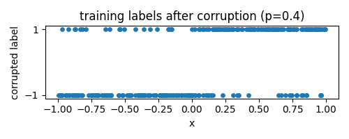
We consider models of the form $f : [-1,1] \to \mathbb{R}^2$, with prediction determined by $\arg\max_i f_i(x)$. We fix an architecture that can in principle interpolate the training data for all $p$.

A linear model would not be enough. If $f$ is affine, then the decision rule depends on the sign of $f_2(x) - f_1(x)$, which is itself affine. Such a function can change sign at most once on $[-1,1]$, and therefore cannot fit arbitrarily many label alternations.

We therefore need a nonlinear model. A piecewise affine function with sufficiently many pieces is enough. We use a one-hidden-layer network with ReLU activations, wide enough to interpolate even at $p=1$. As $p$ increases, the function must oscillate more and more to fit the training data. Each hidden unit introduces one breakpoint: $x \mapsto \sigma(wx + b)$ changes slope at $-b/w$.

We aim to train until near interpolation, so the generalization gap is simply the population error.

What should the population error be?

On the $p$ fraction of corrupted labels: nothing beats random guessing, and population error there should be $1/2$. On the $1-p$ fraction of clean labels: the sign function is optimal, with error $0$. So the best possible population error we can observe, called Bayes error, is:

Now let’s see what happens in practice (results below).

run the next code in Google colab (~4 minutes on CPU)

import numpy as np, torch
import torch.nn as nn, torch.nn.functional as F
import matplotlib.pyplot as plt

torch.manual_seed(0)
rng_xtr = np.random.default_rng(4)
rng_xte = np.random.default_rng(5)     # different RNGs for train/test/corruption: so if we increase n_train or n_test, inputs and corrupted labels for first n_train/n_test points does not change (otw consumes more RNG calls)
rng_ytr = np.random.default_rng(6)
rng_yte = np.random.default_rng(7)

n_train, n_test = 32, 1000 # n_test large enough to sample [-1,1] with high resolution and get accurate population error estimate
width = 1024  # wide enough to interpolate at p=1 (n_train << width)
ps = np.linspace(0, 1.0, 11) # label corruption levels to sweep over

epochs=100_000
lr=1e-3

early_stop = True
nb_errors_allowed = 0               # early stop if <= this many errors
freq_check = 100                     # check early stop every freq_check epochs

train_err, test_err = [], []

for p in ps:
    # data = {(x, y)} with x~Unif([-1,1]), y = sign(x) with proba 1-p, y = Unif({0,1}) otw
    xtr = rng_xtr.uniform(-1, 1, (n_train, 1)).astype(np.float32)
    ytr = (xtr[:, 0] > 0).astype(np.float32)[:, None]

    xte = rng_xte.uniform(-1, 1, (n_test, 1)).astype(np.float32)
    yte = (xte[:, 0] > 0).astype(np.float32)[:, None]

    # corrupt train and test labels: pick exactly ceil(p * n_train) labels y to replace with Unif({0, 1})
    mask_ytr = rng_ytr.choice(n_train, size=int(np.ceil(p * n_train)), replace=False)
    mask_yte = rng_yte.choice(n_test, size=int(np.ceil(p * n_test)), replace=False)
    if mask_ytr.size > 0:
        ytr[mask_ytr] = rng_ytr.integers(0, 2, mask_ytr.size).astype(np.float32)[:, None]
    if mask_yte.size > 0:
        yte[mask_yte] = rng_yte.integers(0, 2, mask_yte.size).astype(np.float32)[:, None]

    xtr = torch.tensor(xtr)
    ytr = torch.tensor(ytr, dtype=torch.long).squeeze()
    xte = torch.tensor(xte)
    yte = torch.tensor(yte, dtype=torch.long).squeeze()


    net = nn.Sequential(nn.Linear(1, width), nn.ReLU(), nn.Linear(width, 2))
    opt = torch.optim.Adam(net.parameters(), lr=lr)

    # train until (almost) perfect fit
    for t in range(epochs):
        opt.zero_grad()
        logits = net(xtr)
        loss = F.cross_entropy(logits, ytr)
        loss.backward()
        opt.step()

        if early_stop and (t % freq_check == 0):
            with torch.no_grad():
                tr_err_now = (net(xtr).argmax(dim=1) != ytr).float().sum().item()
            if tr_err_now <= nb_errors_allowed:
                break

    with torch.no_grad():
        tr_err = (net(xtr).argmax(1) != ytr).float().mean().item()
        te_err = (net(xte).argmax(1) != yte).float().mean().item()

    train_err.append(tr_err); test_err.append(te_err)

plt.figure(figsize=(5,3))
plt.plot(ps, train_err, "o-", label="train")
plt.plot(ps, test_err, "o-", label="population")
plt.axhline(0.5, ls="--", color="gray", label="random chance")
plt.plot(ps, ps/2, "k--", label="Bayes optimal")  # Bayes error = p/2
plt.xlabel("label corruption p")
plt.ylabel("error")
plt.title("train/population error vs label corruption")
plt.ylim(-0.05, 1.05)
plt.legend()
plt.tight_layout()
plt.show()

what happens: model fits everything, population error depends on data

We obtain the next plot.

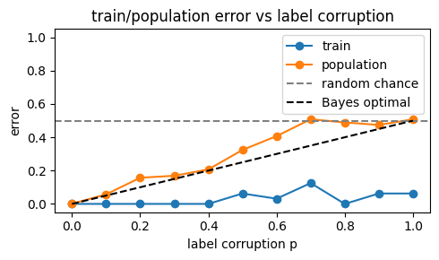
Two observations:

• train error is near 0 for all $p$: the model fits everything, even pure noise;
• population error tracks the Bayes error $p/2$.

Same model, same optimizer, but different data (here, data with different corruption levels) leads to different generalization.

This is a simple illustration of what is discussed in
Understanding Deep Learning Requires Rethinking Generalization (Zhang et al., 2016).

why this matters: ruling out certain complexity measures

Suppose a bound of the form:

Suppose the complexity measure does not depend on the labels. Then it must upper bound the generalization gap for all possible label assignments, including completely corrupted ones. But in that case, no model can beat random guessing. Because the complexity term does not depend on the labels, once it is forced to be at least 1/2 in the fully corrupted case, it is at least 1/2 for every dataset. The bound is therefore uninformative. Let us see this in more detail.

From the experiment we have:

for all $p$. If the complexity term is independent of $p$, it must bound this gap from above for $p=1$. In other words, it must work even when the labels are completely random. That implies:

for all $p$, even in the uncorrupted case $p=0$. The bound is therefore uninformative, since an error of $1/2$ corresponds to random guessing. This argument goes beyond this specific example: if the same model + optimizer can fit arbitrarily reassigned labels in a classification problem, then any data-independent complexity measure must be at least the error of random guessing.

This includes complexity measures such as VC dimension and Rademacher complexity, which quantify the expressive power of a hypothesis class, sometimes in a distribution-dependent way through the inputs, but independently of the labels being fitted and the optimization process. In the present setting, the class is rich enough to fit arbitrary label assignments. These quantities are therefore necessarily large and yield uninformative bounds. A smaller, data-dependent subclass could in principle have lower complexity, but the conclusion remains that the input-label distribution must enter the explanation.

takeaway

If a model + optimizer can fit anything, then generalization cannot be explained without the data.

This may sound tautological: if generalization changes with the data, then the data must be part of the explanation.

Many models and optimizers used in practice fall into this category, as emphasized by Zhang et al. (2016).

This does not tell us the right complexity measure. It tells us which ones cannot work, even in one dimension.

reference

Chiyuan Zhang, Samy Bengio, Moritz Hardt, Benjamin Recht, Oriol Vinyals. Understanding Deep Learning Requires Rethinking Generalization. 2016. arXiv:1611.03530

cite this post as:

@misc{gonon2026data-dependence-generalization,
  title  = {Same Model, Same Optimizer -- Different Generalization},
  author = {Antoine Gonon},
  year   = {2026},
  url    = {https://dimension-one.github.io/blog/2026-02-16-data-dependence-generalization/}
}