minimal sharpness and l2 norm at stable learning rates, edge of stability at the largest ones
with Andreea-Alexandra Mușat, Javier Maass Martinez, and Nicolas Boumal
When many parameters give zero loss, GD still picks one.
A whole line of work studied which implicit bias GD has in such cases. A simple example is linear least squares started at zero, where GD converges to the minimum l2-norm solution see Bach’s lecture notes on implicit bias of GD. Another possible bias is toward lower sharpness. Sharpness is, in its simplest form, the maximum eigenvalue of the Hessian at a given point. (The flatness concept is related: lower sharpness means flatter). This says something about the curvature of the loss: lower sharpness means the loss changes less under small parameter perturbations.
Another line of work says that GD operates at the edge of stability on ML objectives. This refers to the observation that in many ML runs, the sharpness oscillates around $2/\eta$, where $\eta$ is the learning rate. This has caught attention because a second-order local Taylor picture cannot explain it. Indeed, for an exact quadratic, it is impossible to oscillate around the edge of stability: crossing $2/\eta$ means no going back, the dynamics will diverge. In neural networks, the sharpness can go above the edge and then come back. This calls for proof techniques that go beyond classical second-order local analysis.
Here, we look at which regime shows up on the same non-convex 1-hidden linear neuron as in the previous post.
$$ L(x,y)=\frac12(1-xy)^2. $$Does GD converge near minimal sharpness, minimal l2 norm or edge of stability?
The minimizers are
$$ xy=1. $$At a minimizer, the Hessian eigenvalues are
$$ 0 \qquad\text{and}\qquad x^2+y^2. $$details (click to expand): why these are the Hessian eigenvalues
The gradient is
$$ \nabla L(x,y) = \begin{pmatrix} y(xy-1)\\ x(xy-1) \end{pmatrix}. $$So the Hessian is
$$ \nabla^2 L(x,y) = \begin{pmatrix} y^2 & 2xy-1\\ 2xy-1 & x^2 \end{pmatrix}. $$At a minimizer, $xy=1$. So
$$ \nabla^2 L(x,y) = \begin{pmatrix} y^2 & 1\\ 1 & x^2 \end{pmatrix}. $$Its determinant is $x^2y^2-1=0$. Its trace is $x^2+y^2$. So the eigenvalues are $0$ and $x^2+y^2$.
The zero direction is tangent to $xy=1$. Indeed, $(x,-y)$ is tangent and the Hessian sends it to zero.
The zero eigenvalue is tangent to the minimizer curve. The other one is curvature across the curve. Call it $s(x,y)$:
$$ s(x,y):=x^2+y^2. $$It coincides with the sharpness only on the minimizer curve (otherwise, the Hessian eigenvalues are different), so it is a good proxy for sharpness only in the late phase of the runs, once they are already close to the minimizer curve.
This is also the squared l2 norm of the parameters:
$$ s(x,y)=x^2+y^2=\|(x,y)\|_2^2. $$The minimum is $s=2$. It is reached at the minimizers which are balanced ($x=y$). So here, an implicit bias toward minimal sharpness is also an implicit bias toward minimal l2 norm.
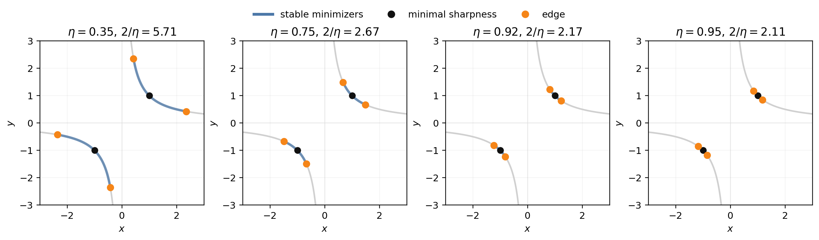
As seen in the previous post, a minimizer can be stable only if
$$ 0< \eta s(x,y)<2 $$
Since $s(x,y)\geq 2$ on $xy=1$, this already requires $0<\eta<1$.
As $\eta$ increases, the sets of stable minimizers shrink around the balanced ones, where sharpness is minimal.
Generically, if GD converges on this loss, it has to converge to a minimizer satisfying the GD stability bound $\eta s(x,y)\le 2$.
details (click to expand): why GD can only converge to a stable minimizer
See for instance Proposition 3.1 in Bolte, Le and Pauwels, 2025: for a $C^2$ semi-algebraic loss, for almost every learning rate $\eta$ and initialization, if GD converges to a point, then every Hessian eigenvalue $\lambda$ at the limit satisfies
$$ 0 \leq \lambda \leq \frac{2}{\eta}. $$Our loss is polynomial, hence $C^2$ and semi-algebraic. If a GD sequence converges, its limit is a critical point. Here the critical points are the saddle $(0,0)$ and the minimizer curve $xy=1$.
At $(0,0)$, the Hessian is
$$ \begin{pmatrix} 0 & -1\\ -1 & 0 \end{pmatrix}. $$Its eigenvalues are $-1$ and $1$. So the saddle violates $\lambda\geq 0$. It is excluded for almost every initialization.
On the minimizer curve, the Hessian eigenvalues are $0$ and $s(x,y)$. The condition becomes
$$ \eta s(x,y) \leq 2. $$So, among these stable minimizers, where does GD actually end?
what we record
We run GD from a deterministic $141\times 141$ grid of starts, masked to the disk $x^2+y^2\leq 9$.
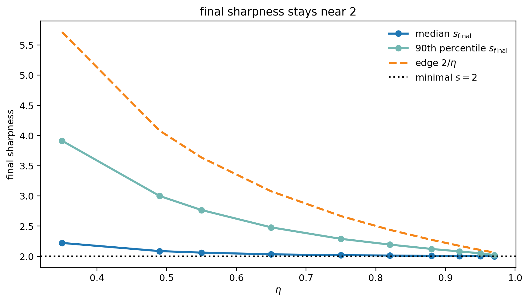
For each convergent run, we record
$$ s_{\mathrm{final}}=s(x_{\mathrm{final}},y_{\mathrm{final}}), $$The next plot shows that the median final sharpness (equivalently, the median final l2 norm) stays near the minimum $s=2$ for all tested stable learning rates.
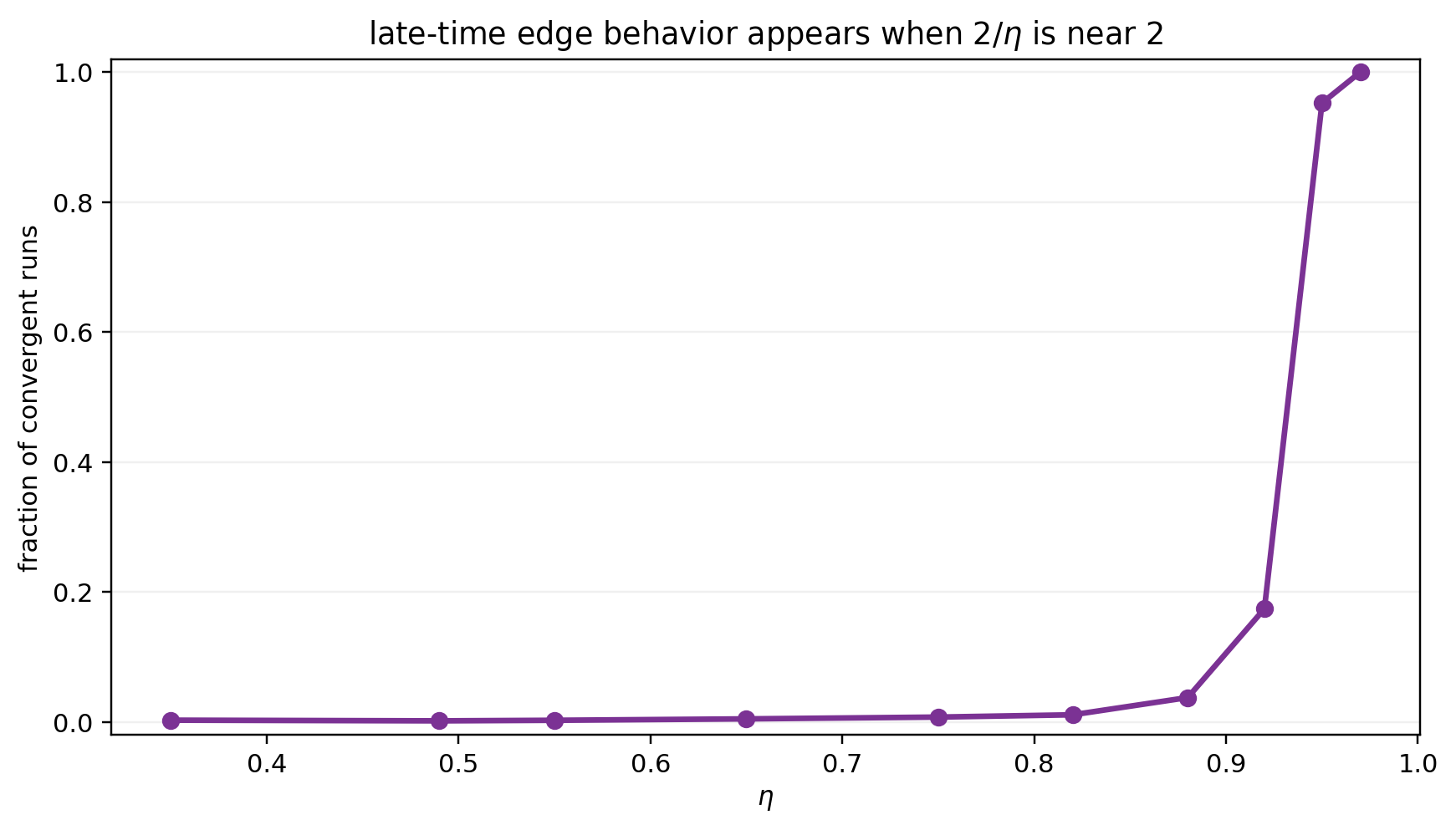
We also measure the proportion of runs that have spent time near the edge of stability, defined as runs for which the median gap over iterations satisfies $|\eta s(x,y)-2|<0.1$ in the late steps of the run, once $|xy-1|$ has dropped below $1\%$ of its initial value. The next plot shows that almost no run spends time near the edge of stability according to this criterion for learning rates $\eta<0.9$, and this fraction increases to almost 1 when $\eta$ gets close to the stability boundary $\eta=1$.
Remember that $s(x,y)=x^2+y^2$ is exactly sharpness only on the minimizer curve $xy=1$. This remains a good proxy close to the minimizer curve. Using the exact sharpness instead gives the same qualitative picture in this late-minimizer regime.
So the observation is:
- minimal sharpness (or l2 norm) shows up across the tested stable range
- runs with sharpness near the edge $2/\eta$ only show up near the largest stable learning rates
is the picture biased by the choice of the initialization region?
We verify whether changing the initialization region changes the picture: maybe considering a square, diamond, or annulus instead of a disk would change the median final sharpness.
The next plot shows for different learning rates $\eta$ the final sharpness from each grid point in the disk $x^2+y^2\leq 9$. We use a uniform $141\times 141$ grid in $(x_0,y_0)$, clipped to the disk.
Gray means no convergence in the step budget. White curves share the same imbalance $x^2-y^2$.
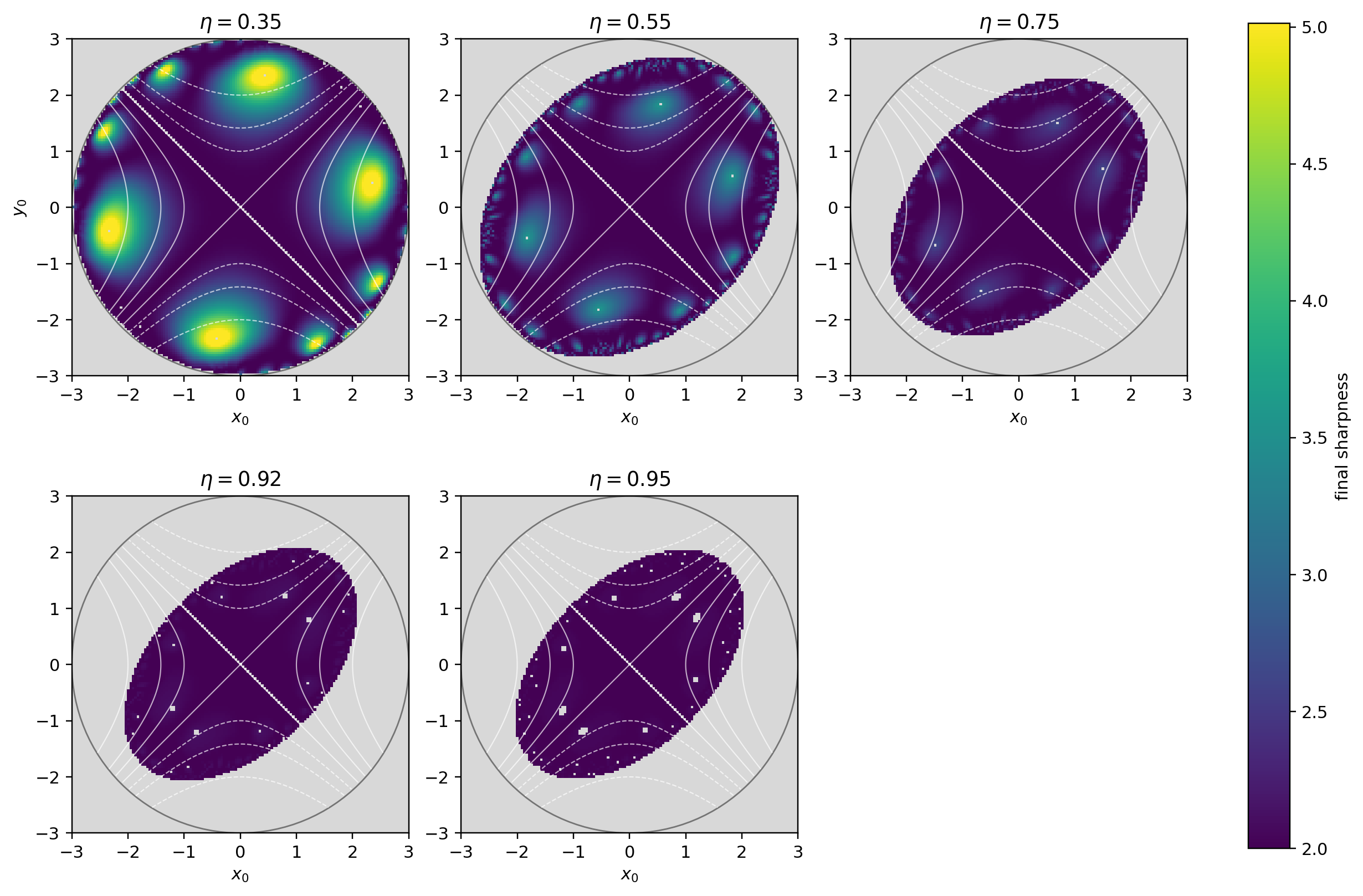
No regular shape seems specifically advantaged here. The regions from which GD does not end near minimal sharpness look irregular. So changing from disk to another regular shape does not seem enough to move the median away from minimal sharpness.
The notebook repeats this on the same kind of uniform grid for a square, diamond, and annulus. The medians stay near $2$ (exact values depend on the shape, but the qualitative picture is the same).
Note that this drift toward minimal sharpness / l2 norm is a finite-step GD effect, not a gradient-flow effect, because gradient flow preserves the imbalance $x^2-y^2$ (see details below) so the dynamics cannot favor the balanced minimizers. So we should have expected in the first place that minimal sharpness / l2 norm cannot uniformly appear across all learning rates: small learning rates are closer to gradient flow, so they should show less bias toward balanced minimizers. This is what we observe above. Another takeaway is that already on this simple loss, gradient flow misses two phenomena discussed in ML optimization. It misses implicit bias toward minimal sharpness / l2 norm. It also misses edge of stability behavior.
details (click to expand): why gradient flow preserves imbalance, but GD does not
Gradient flow is
$$ \dot x = y(1-xy), \qquad \dot y = x(1-xy). $$So
$$ \frac{d}{dt}(x^2-y^2) = 2x\dot x-2y\dot y = 2xy(1-xy)-2xy(1-xy) =0. $$For GD,
$$ x_{k+1}=x_k-\eta y_k(x_ky_k-1), \qquad y_{k+1}=y_k-\eta x_k(x_ky_k-1). $$A direct computation gives
$$ x_{k+1}^2-y_{k+1}^2 = (x_k^2-y_k^2)\left(1-\eta^2(x_ky_k-1)^2\right). $$So finite-step GD slowly changes the imbalance. The effect becomes weaker as $\eta\to 0$.
The next plot is interactive. Choose a learning rate by sliding the top bar. Then click a point on the left panel to see the GD trajectory and sharpness evolution for that initialization in the right panels.
run in Google Colab (CPU is enough)
takeaway
For this simple loss, GD empirically ends up near the balanced minimizers for stable learning rates. Here this means near minimal sharpness / l2 norm. One may say this is a possible form of implicit bias (note that we did not observe exact minimal sharpness, but rather a concentration near it).
Near the largest stable learning rates, the balanced minimizers are also near the edge of stability. For this simple loss, we would not see this edge-related behavior without larger learning rates.
references
For flatness and sharpness:
For implicit bias and minimum l2 norm:
For edge of stability:
cite this post as:
@misc{gonon2026minsharpeos,
  title  = {Minimal Sharpness and L2 Norm at Stable Learning Rates, Edge of Stability at the Largest Ones},
  author = {Antoine Gonon and Andreea-Alexandra Mușat and Javier Maass Martinez and Nicolas Boumal},
  year   = {2026},
  url    = {https://dimension-one.github.io/blog/2026-06-15-minimum-sharpness-stable-learning-rates-eos/}
}