← home

a phase portrait of gradient descent on a 1-hidden linear neuron

May 18, 2026

with Andreea-Alexandra Mușat, Javier Maass Martinez, and Nicolas Boumal

Take the smallest factorized linear model: one hidden linear neuron, with input weight $x$ and output weight $y$. For an input sample equal to $1$, the model predicts $1 \cdot xy = xy$.
If the target value is $1$, then the least-squares error is

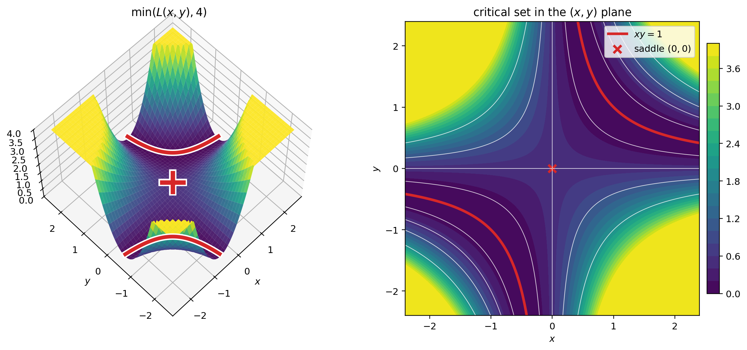
The prediction is bilinear in the parameters, so the loss is quartic and non-convex: $L(1,1)=L(-1,-1)=0$, but $L(0,0)=1/2$. The zero-loss points are not isolated either. They form the hyperbola

This is a toy loss, but it already has a continuous curve of minimizers and is the simplest version of factorized losses used in matrix factorization and deep linear networks. More on this at the end.

The question is:

for a fixed learning rate, what does GD do from each initialization?

More precisely: does it reach $xy=1$, settle at the saddle $(0,0)$, or diverge? And if it reaches $xy=1$, does it cross that curve before settling?

behavior of gradient descent from initializations in $[-3,3]^2$

The next figure shows, for each initialization in $[-3,3]^2$, what gradient descent does when started from that point, with one panel for each learning rate $\eta$.

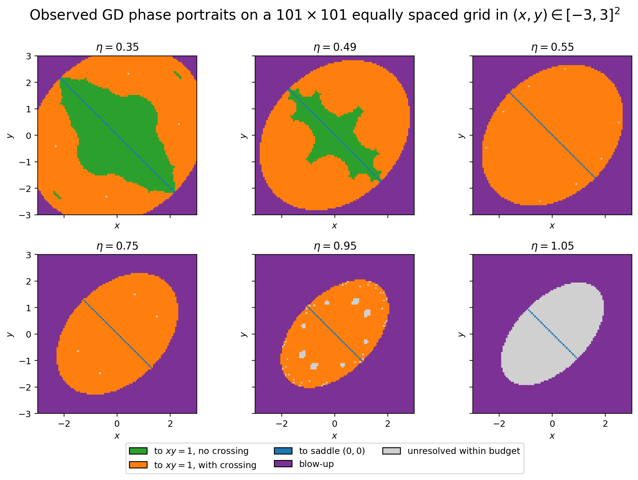
Each pixel is an initialization in $[-3,3]^2$. The colors mean:

• green: reaches $xy=1$ without crossing it,
• orange: reaches $xy=1$ with at least one crossing,
• blue: settles at the saddle $(0,0)$,
• purple: diverges,
• gray: unresolved within the step budget.

The displayed sweep already shows the two transitions. The green region disappears between $\eta=0.49$ and $\eta=0.55$. The visible region reaching $xy=1$ disappears between $\eta=0.95$ and $\eta=1.05$. Refining the sweep gives the exact thresholds

The value of this example is that everything is visual. The message is standard: when $\eta$ increases, the stable part of the minimizer set (i.e., the part that is locally attractive) shrinks. This happens because, near a minimizer, gradient descent behaves at first order like a linear dynamical system: at each step, it multiplies the distance to the minimizer by a factor depending on the learning rate and the local geometry of the loss. For local attraction to hold, this factor must stay below one in absolute value, and since it grows with $\eta$, there are fewer and fewer points on the minimizer curve that can attract nearby trajectories, and eventually none at all.

Here we derive this without special machinery, using one coordinate across xy=1 and one coordinate along it. At the end of the post, we return to the same computation for a general smooth loss with a smooth valley of minimizers. Depending on one’s background, this can be phrased using a local PŁ/error-bound/quadratic-growth or a Morse-Bott condition. A different derivation uses the center-stable manifold theorem from dynamical systems. Here, we will stick to the most elementary version: local tangent/normal coordinates and Taylor expansion.

This post focuses only on explaining these learning-rate thresholds, which come from the late-stage behavior near the minimizer curve. In practice, a more interesting question is what happens before these local coordinates become accurate: this earlier phase determines where the dynamics eventually settle on the minimizer set, and can influence properties such as flatness or edge-of-stability behavior of the final solution. That will be for next time.

The plot uses a $101\times101$ grid in $[-3,3]^2$ and runs GD for at most $320$ steps. The exact labeling code is in the Colab.

run in Google Colab (a few seconds on CPU)

You can also explore the same picture interactively, point by point. Feel free to click on the right panel to display the trajectory from a chosen initialization, change the learning rate, or rotate the loss surface shown on the left panel:

Plan. To explain the picture, we discuss three points: where GD can settle, how GD moves near the zero-loss curve, and why the two thresholds are one half and one. And as a complement, at the end of the post, we show how the same considerations apply to a general smooth loss: the learning-rate thresholds can be read directly from the linearized gradient descent dynamics near the minimizer curve.

where GD can settle ↩ plan

GD only stops when the gradient is zero, that is, at critical points of the loss.

For this loss, the critical points are either the global minimizers satisfying $xy=1$, or the saddle point $(0,0)$.

Indeed, the gradient is

which vanishes only in these two cases.

To see that the origin is a saddle point (meaning that one can move away from it either by increasing or decreasing the loss), consider a small nonzero $\varepsilon$. Then

coordinates near the minimizer curve ↩ plan

To understand crossing and attraction near $xy=1$, we introduce coordinates adapted to this curve. We want one coordinate for motion across the curve, and one coordinate for motion along it. The choice below is not unique, but it is simple and makes the GD update easy to read.

The minimizers are exactly the points satisfying

This suggests the across-curve coordinate

Then crossing the minimizer curve means changing the sign of $n$. Geometrically, $n$ measures displacement across the curves $xy=\text{constant}$.

We also introduce a coordinate that varies along these curves. Since

is normal to the curves $xy=\text{constant}$, a tangent direction is given by any perpendicular vector. One simple choice is

A convenient scalar coordinate associated with this direction is

Indeed,

which is parallel to $(x,-y)$. Thus, to first order, $t$ varies along the curves $xy=\text{constant}$, while $n$ varies across them.

Note that the $t$ coordinate measures imbalance between the two factors, with $t=0$ at perfectly balanced minimizers satisfying $x=y$.

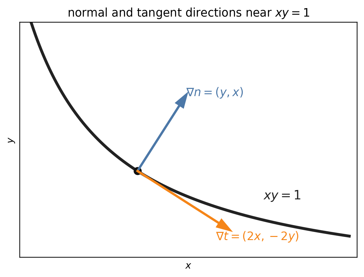
The picture shows this at one point on $xy=1$: $\nabla n=(y,x)$ is normal to the curve, while $\nabla t=(2x,-2y)$ is tangent to it.

In these coordinates, one GD step on $(x_k,y_k)$ induces the following update on $(t_k,n_k)$:

and

The first equation shows that near the minimizer curve, where $n_k$ is small, $t_k$ barely changes:

So once the trajectory is close to $xy=1$,
the trajectory mostly moves across the curve, not along it.

For the normal coordinate, keeping only the leading term gives

Thus the local behavior (attractive or repulsive) near the minimizer curve is controlled by the factor $1-\eta s(t_k)$, and we discuss below how it relates to the colors in the phase portrait at the beginning of the post.

Here, crossing means crossing the hyperbola $xy=1$, equivalently changing the sign of $n=xy-1$.

This gives a local explanation of the colors in the phase portrait, which is enough to understand the two transitions at $\eta=1/2$ and $\eta=1$ (see next section).

The green region must satisfy the first condition, since it must converge to $xy=1$ without crossing it, but is usually only a subset of that condition, because crossing may already have happened during the early steps, before the local approximation applies.

All points satisfying the second condition are orange, because they cross the minimizer set once they are close enough to it (except if they land exactly on the curve before crossing, let’s ignore those pathological cases for simplicity).

Finally, points satisfying the third condition are gray or purple, because they are locally repelled from the minimizer curve (up to pathological cases).

why the thresholds are one half and one ↩ plan

Along the zero-loss curve, the quantity controlling the local behavior of gradient descent is

Its smallest possible value is

which is reached at the balanced minimizer $x=y$.

To converge toward $xy=1$ without oscillating across the curve, we need

Since $s(t)\ge 2$, this can only happen if

This explains why the green region disappears at $\eta=\frac12$: beyond this value, even the most stable minimizer cannot attract nearby points without crossings.

More generally, to attract nearby points at all, we need

Again using $s(t)\ge 2$, this requires

This is why the curve $xy=1$ stops attracting nearby points when $\eta=1$.

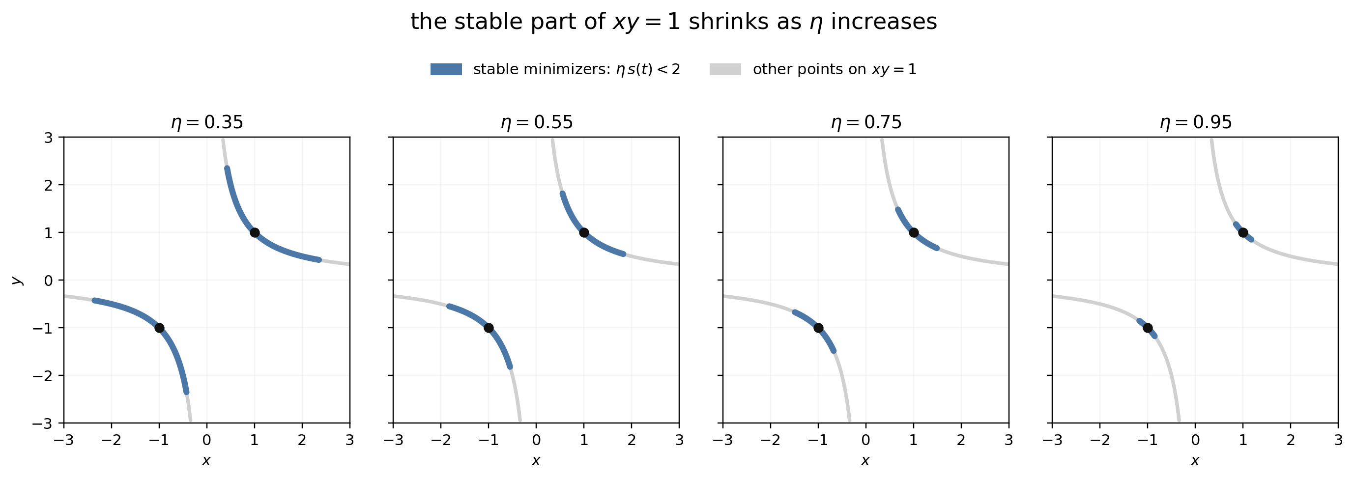
For $\eta<1$, the attracting part of the curve is exactly

As $\eta$ increases, this stable part shrinks toward the balanced minimizer and disappears completely at $\eta=1$.

The next figure shows only this stable part of $xy=1$ in blue; the rest of the minimizer curve is gray.

where this toy example sits ↩ plan

The loss

is the simplest member of a hierarchy of factorized losses.

If we replace the scalars by matrices, we obtain matrix factorization (a.k.a. one-hidden linear network):

If we replace the single product by a product of several matrices, we obtain deep linear networks:

The scalar case already keeps several features of the larger problems: non-convexity, a continuous surface of parameters representing the same prediction, hence a continuous curve of minimizers and different behavior at different points on that curve.

The advantage here is that everything remains two-dimensional, so the full phase portrait can be visualized directly. Of course, higher-dimensional models can behave differently.

takeaway

The two special learning rates come from the same late-stage behavior near $xy=1$:

So the behavior of gradient descent near the minimizer set is controlled by the local multiplier $\eta(t^2+4)^{1/2}$.

As the learning rate increases, there are fewer values of $t$ for which this multiplier is smaller than one. These are exactly the points where the minimizer curve can attract nearby trajectories without crossings.

This possibility disappears at $\eta=1/2$: even the balanced minimizer, which has the smallest possible multiplier, can no longer attract nearby points without oscillations across the curve.

If the learning rate increases further, there are also fewer values of $t$ for which the multiplier is smaller than two. These are the points where the minimizer curve can attract nearby trajectories at all.

This attraction disappears completely at $\eta=1$: even the balanced minimizer can no longer pull nearby points inward, and instead repels them.

cite this post as:

@misc{gonon2026phaseportraitgdlinear,
  title  = {A Phase Portrait of Gradient Descent on a 1-Hidden Linear Neuron},
  author = {Antoine Gonon and Andreea-Alexandra Mușat and Javier Maass Martinez and Nicolas Boumal},
  year   = {2026},
  url    = {https://dimension-one.github.io/blog/2026-05-18-phase-portrait-gradient-descent-linear-neuron/}
}

complement: same local picture for a smooth loss ↩ plan

Below, we explain why the computation above is not specific to

Given a smooth loss that is essentially flat along a smooth set of minimizers, and quadratic along the normal directions (Morse-Bott assumption), gradient descent decomposes into a slow tangent motion and a fast normal motion. To first order, GD updates only the normal coordinate: $n_{k+1}=(I-\eta H(t_k))n_k$, where $H(t)$ is the Hessian restricted to the normal space at the point with tangent coordinate $t$. Thus, if $\lambda_{\max}$ is the largest eigenvalue of $H(t)$, a minimizer is locally stable iff $0<\eta \lambda_{\max}<2$, and non-oscillatory iff $0<\eta\lambda_{\max}<1$, giving again two learning-rate thresholds. We now derive this in detail, assuming a minimalist background (Taylor expansion, inverse function theorem, and the definition of a manifold).

Let

be a smooth loss, and suppose that, the minimizers form a smooth manifold

$S$ is the analogue of the curve $xy=1$. Moving along $S$ does not change the loss. Moving away from $S$, in a direction transverse to it, and we will assume it increases the loss quadratically.

Let $r$ be the codimension of $S$. This means that, locally, $S$ has dimension $d-r$, and there are $r$ independent directions in which one can move away from it. In the toy example, $d=2$, the minimizer set $xy=1$ is one-dimensional, and therefore $r=1$.

The assumption we make is the following. At each minimizer $w_\star\in S$ near the point under consideration, the kernel of the Hessian is exactly the tangent space to the minimizer set:

and the Hessian is positive definite in the directions normal to $S$.

In words: the loss is flat along the valley of minimizers, but has positive quadratic curvature across it.

In technical terms, the loss satisfies a Morse-Bott property. For $C^2$ losses, it is also equivalent to local PŁ/error-bound/quadratic-growth conditions near the minimizer set, see Rebjock and Boumal (2024) for precise statements. Here we only use the elementary consequence we need: near $S$, we can choose coordinates that separate directions along the valley from directions across the valley, and show that the loss is quadratic in the normal directions.

We now introduce coordinates playing the same role as $t$ and $n$ in the toy example.

Because $S$ is a smooth manifold of dimension $d-r$, around any point of $S$ we can parametrize it by $d-r$ real numbers (i.e., there is a smooth map from an open subset of $\mathbb R^{d-r}$ to $S$ that is a diffeomorphism onto its image). Write this parametrization as

Thus $t$ is the tangent coordinate: it labels which minimizer on $S$ we are close to.

At each point $p(t)$, the tangent space $T_{p(t)}S$ has dimension $d-r$. Its orthogonal complement, the normal space, has dimension $r$. Choose an orthonormal basis of this normal space and put its vectors in the columns of a matrix

So the columns of $Q(t)$ span the directions across the valley at $p(t)$.

There is a small standard useful fact here: this normal basis can be chosen smoothly, after shrinking the neighborhood if necessary. One way to see it is the following. The columns of $Dp(t)$ form a smooth basis of the tangent space. Therefore the orthogonal projection onto the tangent space,

depends smoothly on $t$. So the normal projection $P_N(t)=I-P_T(t)$ is also smooth. Since its rank is constantly $r$, we can locally choose $r$ fixed coordinate vectors whose projections by $P_N(t)$ remain independent, and then apply Gram-Schmidt. This gives a smooth orthonormal normal frame $Q(t)$.

Now let

be the normal coordinate. The nearby point with tangent coordinate $t$ and normal coordinate $n$ is

This map $(t,n)\mapsto p(t)+Q(t)n$ gives valid coordinates locally.
At $n=0$, its differential with respect to $(t,n)$ is the linear map

Its tangent columns come from $Dp(t)$, and its normal columns come from $Q(t)$. Together, these columns form a basis of $\mathbb R^d$. Thus the derivative is invertible, and the inverse function theorem says that, after shrinking the neighborhood if necessary, every nearby point can be written uniquely as

In these $(t,n)$ coordinates,

So $t$ and $n$ are the general versions of the two coordinates used above: $t$ moves along the valley, and $n$ moves across it.

In the toy example, the tangent coordinate was

and the across-curve coordinate was

The only small difference is that now, in the general case, $n$ is a Euclidean normal displacement after locally “straightening” the manifold. By contrast, in the toy examplem, we did not bother to straighten the curve in the toy example and chose $n=xy-1$ instead. We did that for simplicity since it was enough to get the same local picture (straightening the curve would have just changed the normal coordinate by a smooth scaling factor, giving the same sign flips, hence the same crossings, and the same first-order contraction factor in the normal direction).

Now expand the loss in these coordinates. Since every $p(t)$ is a minimizer,

Taylor expansion in the normal variable gives

where

is the Hessian restricted to the normal space.

By the nondegenerate-valley assumption, $H(t)$ is positive definite. Thus, to leading order, the loss is a quadratic least-squares-like loss in the normal variable. So the local picture is the same as in the toy example: the loss is flat along the valley and quadratic across the valley. If one invokes the Morse-Bott lemma, one can even choose local coordinates in which this quadratic normal form is exact. For the GD calculation below, however, the leading Taylor term is enough.

Now run gradient descent:

Write

Taylor expansion of the gradient at $p(t_k)$ gives, using the fact that $\nabla L(p(t_k))=0$,

We now use the Hessian structure at a minimizer. Since $\nabla^2L(p(t))$ is symmetric and

the image of $\nabla^2L(p(t))$ is orthogonal to $T_{p(t)}S$. In other words, it lies in the normal space and $\nabla^2L(p(t))Q(t)n$ is a normal vector. Because the columns of $Q(t)$ form an orthonormal basis of the normal space, projecting onto this basis gives

Thus

So, to first order, the gradient points purely in the normal direction. It has no tangent component of order $\|n_k\|$.

One GD step therefore gives

The leading term is already written in our local coordinates: it has tangent coordinate $t_k$ and normal coordinate $(I-\eta H(t_k))n_k$.

Since the inverse coordinate map is smooth, the remaining $O(\|n_k\|^2)$ perturbation in parameter space only creates an $O(\|n_k\|^2)$ perturbation in coordinate space. Therefore, the new coordinates $(t_{k+1},n_{k+1})$ of $w_{k+1}$ satisfy

In particular, to first order, GD moves across the valley, not along it, and the leading normal dynamics is linear, with multiplier $I-\eta H(t_k)$.

This is exactly what happened for

There, we found the exact identity

so the tangent coordinate $t=x^2-y^2$ changes only at second order in the across-curve coordinate $n=xy-1$. The general formula

is the same statement.

Now suppose that a GD trajectory converges to some minimizer

Once the trajectory is close to this minimizer, $H(t_k)$ is close to $H(t_\infty)$, so the leading normal dynamics is

Let

be the eigenvalues of the Hessian $H(t_\infty)$ restricted to the normal space (these are positive by the nondegenerate-valley assumption). Along a normal eigenvector, the update is approximately multiplication by

Thus the minimizer can be locally attractive only if every normal component contracts:

Equivalently,

In other words,

For attraction without local oscillations in the normal direction, we need the stronger condition

or equivalently

In codimension one, a sign flip of the normal coordinate is literally a crossing of the minimizer set. In higher codimension, there are several normal directions. The same statement applies along each normal eigenvector: components with

contract while alternating sign, while components with

are locally repelled.

The equality case $\eta\lambda_i=2$ is borderline and higher-order terms matter, so the clean local attraction statement uses strict inequalities.

This recovers the same picture as in the toy example: as the learning rate increases, fewer minimizers satisfy these inequalities, and the stable part of the minimizer set shrinks toward the most stable point.

This local analysis explains which minimizers are stable for a given learning rate, but not which stable minimizer a trajectory reaches. That choice is made before the trajectory enters the regime where these local coordinates become accurate. More on that in the next post.